Jaxonomy — hybrid dynamical systems on JAX MCP Server

<div align="center"> <img src="https://raw.githubusercontent.com/machinavitalis/jaxonomy/main/docs/examples/media/hero_triptych.gif" width="100%" alt="Jaxonomy — compose, simulate, control">

Jaxonomy

Differentiable simulation of hybrid dynamical systems — powered by JAX.

Block diagrams meet automatic differentiation. Model physical systems, close the loop with LQR/MPC/Kalman, and differentiate through everything.

Why JAX? · Install · Quick Start · Gallery · Examples · Docs

_{Every panel above is produced by <code>jaxonomy.simulate</code> on a model built from the library.}

</div>

---

What is Jaxonomy?

Jaxonomy is a Python framework for modeling, simulating, and optimizing hybrid dynamical systems — systems that combine continuous physics, discrete control laws, and event-driven logic in a single model. Every simulation runs on JAX, so it is JIT-compilable, batchable with vmap, and fully differentiable from end to end.

import jax.numpy as jnp
import jaxonomy as jx

# Double integrator: A, B, C, D define the plant; Q, R weight the LQR cost.
A, B = jnp.array([[0., 1.], [0., 0.]]), jnp.array([[0.], [1.]])
C, D = jnp.eye(2), jnp.zeros((2, 1))
Q, R = jnp.eye(2), jnp.array([[1.]])

builder = jx.DiagramBuilder()
# Start displaced from the origin, so the regulator has something to do.
plant      = builder.add(jx.library.LTISystem(A, B, C, D,
                                              initialize_states=jnp.array([1.0, 0.0])))
controller = builder.add(jx.library.LinearQuadraticRegulator(A, B, Q, R))
builder.connect(plant.output_ports[0],      controller.input_ports[0])
builder.connect(controller.output_ports[0], plant.input_ports[0])

diagram = builder.build()
results = jx.simulate(
    diagram,
    diagram.create_context(),
    (0.0, 10.0),
    # Nothing is stored unless you name it here: without recorded_signals,
    # results.time and results.outputs come back as None.
    recorded_signals={"x": plant.output_ports[0],
                      "u": controller.output_ports[0]},
)

results.outputs["x"]    # (T, 2) — position and velocity, driven back to zero

---

🔥 Why JAX?

Choosing JAX as the compute backbone unlocks capabilities that are impractical with NumPy-based simulators:

Traditional simulator          Jaxonomy / JAX
──────────────────────         ─────────────────────────────────────────
simulate(params)          →    jit(simulate)(params)          10–100× faster
for p in param_grid: …    →    vmap(simulate)(param_grid)     embarrassingly parallel
finite_diff_gradient(…)   →    grad(simulate)(params)         exact gradients, free

Feature	SciPy / NumPy	Julia / DiffEq	Modelica	MathWorks¹	Jaxonomy
Python-native	✓	✗	✗	✗	✓
JIT / code generation	✗	✓	✓ (C++)	✓ (C/C++)	✓
Full autodiff through ODE	✗	Partial	✗	Partial²	✓
Hybrid events & zero-crossing	Partial	✓	✓	✓	✓
Acausal / equation-based	✗	✗	✓	✓ (Simscape)	✓
Block-diagram composition	✗	Partial	Partial	✓ (Simulink)	✓
State-machine modeling	✗	✗	✗	✓ (Stateflow)	✓
LQR / MPC / Kalman built-in	✗	Partial	Via libs	✓ (Toolboxes)	✓
Neural ODE / SINDy	✗	✓	✗	✗	✓
Reduced-order modeling (balred / POD-DEIM / DMD / Koopman)	✗	Partial	✗	✓ (Toolboxes)	✓
Batch / ensemble (vmap)	✗	✗	✗	✗	✓
Open-source (MIT)	✓	✓	Partial	✗	✓

_{¹ Simulink + Simscape + Stateflow + Control System Toolbox  ·  ² Via Simulink Design Optimization, no end-to-end AD}

---

⚡ Key Capabilities

Capability	What it enables
⚡ JAX-native engine	JIT-compile simulations, run ensembles with vmap, differentiate through ODE solvers including event handling
🔀 Hybrid dynamics + state machines	Continuous ODEs, periodic discrete updates, zero-crossing events, and StateMachineBuilder-authored finite state machines composed in one model. jax.grad flows through event times for hybrid trajectory optimisation.
🔌 Acausal modeling	Modelica-inspired multi-domain components (electrical, mechanical, thermal, fluid, battery) with Pantelides index reduction and a BDF mass-matrix DAE solver
🎯 Control & estimation	LQR (continuous, discrete, finite-horizon, LQG), linear MPC (native + OSQP), nonlinear MPC (shooting / transcription / Hermite-Simpson), Kalman / EKF / UKF / RLS / Luenberger, 2-DOF PID with classical tuning helpers
🧮 Unit-aware wiring	Optional BusUnit annotations on ports and signals; the diagram compiler catches dimensional mismatches at build time instead of as silent runtime bugs
🧠 Data-driven modeling	Neural ODEs, Universal Differential Equations, SINDy symbolic regression, neural-network blocks (MLP / PyTorch / TensorFlow / ONNX), differentiable lookup-table fitting, and statistical surrogates (Gaussian process, polynomial chaos, RBF)
📉 Reduced-order modeling	jaxonomy.library.rom: linear MOR (balanced truncation, minreal, modal / residualization), POD–Galerkin with DEIM hyper-reduction, and data-driven operator ROM (DMD / DMDc / ERA, Koopman / eDMD lifted-linear predictors). One reduce(...) front door; every reduced model is a differentiable, simulatable block
🎲 Uncertainty & sensitivity	First-class jaxonomy.uq workflow: Monte Carlo with parameter distributions, Latin Hypercube + quasi-Monte Carlo sampling, Sobol sensitivity decomposition, Morris screening
🤝 FMI 2.0 / 3.0 interop	Import FMI co-simulation FMUs (ModelicaFMU, mixed-type and array I/O) or model-exchange FMUs (ModelicaFMUME, integrated by Jaxonomy's own solver with FMI event indicators as zero-crossings); export a diagram as a binary .fmu via build_fmu. Verified against the Reference FMUs, OpenModelica, and the fmusim reference simulator in CI
🧩 150+ library blocks	Integrators, filters, state machines, look-up tables, coordinate transforms, container blocks, bus / mux family, stochastic sources, and more

---

📦 Installation

Requires Python 3.10+.

# Create and activate a virtual environment (recommended)
python -m venv .venv
source .venv/bin/activate        # Windows: .venv\Scripts\activate

# Install
pip install jaxonomy             # core
pip install jaxonomy[safe]       # + SciPy, Matplotlib, control, jaxopt
pip install jaxonomy[nmpc]       # + nonlinear MPC (requires IPOPT on PATH)
pip install jaxonomy[all]        # + everything

From source:

git clone https://github.com/machinavitalis/jaxonomy
cd jaxonomy
pip install -e .

CLI runner:

jaxonomy_cli run --model path/to/model.json

---

🚀 Quick Start

A first simulation in a few lines — a custom block, built into a diagram, integrated through its ODE:

import jaxonomy as jx
import jax.numpy as jnp

# Van der Pol oscillator as a custom block
class VanDerPol(jx.LeafSystem):
    def __init__(self, mu=1.0, **kwargs):
        super().__init__(**kwargs)
        self.declare_dynamic_parameter("mu", mu)
        self.declare_continuous_state(
            default_value=jnp.array([0.0, 2.0]), ode=self._ode
        )
        self.declare_continuous_state_output(name="x")

    def _ode(self, time, state, *inputs, **params):
        x, mu = state.continuous_state, params["mu"]
        return jnp.array([x[1],  mu * (1 - x[0]**2) * x[1] - x[0]])

builder = jx.DiagramBuilder()
vdp = builder.add(VanDerPol(mu=2.0, name="vdp"))
diagram = builder.build()

results = jx.simulate(
    diagram, diagram.create_context(), (0.0, 20.0),
    options=jx.SimulatorOptions(buffer_length=4000),  # room for adaptive steps
    recorded_signals={"x": vdp.output_ports[0]},
)
# results.outputs["x"] → time-series of shape (T, 2)

---

📚 Documentation

• Online docs & tutorials: py.jaxonomy.com
• Local docs:

  pip install -r requirements.docs.txt
  mkdocs serve   # → http://127.0.0.1:8000
  

• Example notebooks: docs/examples/
• Scope notes: PINNs & PDE surrogates — classical PDE PINNs are out of scope; physics-informed dynamics learning (UDE / Neural DAE / Neural ODE / SINDy) is core.

---

🤖 Driving Jaxonomy from an AI agent (MCP)

<!-- The line below is the MCP Registry's package-ownership proof. The registry reads it from this README as published to PyPI (pyproject sets readme = "README.md") and requires it to match the "name" in server.json exactly. Do not remove or reword it, and keep it on its own line. --> <!-- mcp-name: io.github.machinavitalis/jaxonomy -->

Jaxonomy ships an MCP server that exposes the engine as tools an AI agent can call directly — it can enumerate library blocks, build and validate a model, run a simulation, fit parameters to data, and linearize a system, then reason over the actual results. This is worth wiring up if you drive Jaxonomy from an agent (Claude Desktop/Code, Cursor, …); if you're writing Python by hand, the pip install above is all you need and you can skip this.

pip install jaxonomy[mcp]

Then register the server with your agent client. For Claude Desktop, add to claude_desktop_config.json:

{
  "mcpServers": {
    "jaxonomy": {
      "command": "python",
      "args": ["-m", "jaxonomy.mcp.server"]
    }
  }
}

Use the interpreter where jaxonomy[mcp] is installed (or the jaxonomy-mcp entry point). The server is listed in the MCP Registry as io.github.machinavitalis/jaxonomy; full tool reference, client configuration and limitations are at py.jaxonomy.com/mcp.

If you'd rather just point an agent at the documentation, start it on SKILL.md — when to use Jaxonomy, when to reach for something else, the core API, and the pitfalls that most often break a first script. The docs site also publishes llms.txt views: py.jaxonomy.com/llms.txt for an index of every page, and py.jaxonomy.com/llms-full.txt for the whole documentation set as one Markdown file.

---

📖 Examples

1 · Hybrid Dynamics: The Bouncing Ball

<div align="center"> <img src="https://raw.githubusercontent.com/machinavitalis/jaxonomy/main/docs/examples/media/grid_bouncing_ball.gif" width="45%" alt="Bouncing ball — hybrid contact events"> </div>

Jaxonomy is designed for hybrid systems — models where continuous physics interacts with instantaneous discrete resets. The bouncing ball is the canonical example: free-fall ODE interrupted by a collision event that reverses velocity.

Governing equations

The dynamics between bounces follow:

$$ \dot{x} = v, \qquad \dot{v} = -g $$

When the ball hits the ground ($x = 0$, $v < 0$) a zero-crossing event fires and the state resets:

$$ x^+ = 0, \qquad v^+ = -e \cdot v \quad (e \in [0, 1] \text{ — coefficient of restitution}) $$

import jaxonomy as jx
import jax.numpy as jnp

class BouncingBall(jx.LeafSystem):
    def __init__(self, g=9.81, e=0.8, **kwargs):
        super().__init__(**kwargs)
        self.declare_dynamic_parameter("g", g)
        self.declare_dynamic_parameter("e", e)
        # [height, velocity]
        self.declare_continuous_state(
            default_value=jnp.array([5.0, 0.0]), ode=self._ode
        )
        self.declare_continuous_state_output(name="state")

        # Zero-crossing: fires as height crosses zero from above
        self.declare_zero_crossing(
            guard=self._hit_ground,
            reset_map=self._bounce,
            direction="positive_then_non_positive",
        )

    def _ode(self, time, state, *inputs, **params):
        v = state.continuous_state[1]
        return jnp.array([v, -params["g"]])

    def _hit_ground(self, time, state, *inputs, **params):
        return state.continuous_state[0]  # guard on height

    def _bounce(self, time, state, *inputs, **params):
        x, v = state.continuous_state
        new_state = jnp.array([0.0, -params["e"] * v])
        return state.with_continuous_state(new_state)

builder = jx.DiagramBuilder()
ball = builder.add(BouncingBall(g=9.81, e=0.85, name="ball"))
diagram  = builder.build()
results  = jx.simulate(
    diagram, diagram.create_context(), (0.0, 8.0),
    recorded_signals={"state": ball.output_ports[0]},
)

Zero-crossing events are located with 40-step bisection on the solver's dense output polynomial — giving sub-microsecond temporal accuracy without user-specified tolerances.

---

2 · Optimal Control: LQR Pendulum

<div align="center">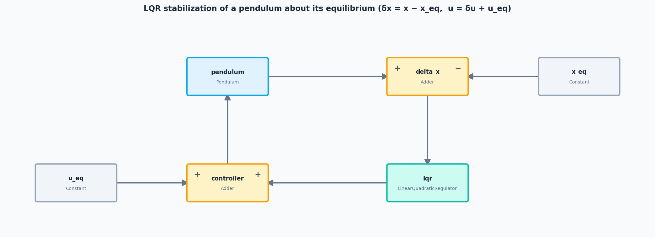

</div>

For a linearized pendulum with state $x = [\theta, \dot\theta]^\top$:

$$ \dot{x} = Ax + Bu, \qquad A = \begin{bmatrix} 0 & 1 \ g/L & 0 \end{bmatrix}, \quad B = \begin{bmatrix} 0 \ 1/mL^2 \end{bmatrix} $$

The Linear Quadratic Regulator minimizes infinite-horizon cost:

$$ J = \int_0^\infty \bigl( x^\top Q, x + u^\top R, u \bigr), dt $$

by solving the algebraic Riccati equation $A^\top P + PA - PBR^{-1}B^\top P + Q = 0$ for the optimal gain $K = R^{-1}B^\top P$, so $u^* = -Kx$.

import jaxonomy as jx
from jaxonomy.library import LTISystem, LinearQuadraticRegulator
import jax.numpy as jnp

g, L, m = 9.81, 1.0, 1.0
A = jnp.array([[0, 1], [g/L, 0]])
B = jnp.array([[0], [1 / (m * L**2)]])
C, D = jnp.eye(2), jnp.zeros((2, 1))

Q = jnp.diag(jnp.array([10.0, 1.0]))  # penalise angle more than rate
R = jnp.array([[0.1]])                 # control effort cost

builder    = jx.DiagramBuilder()
plant      = builder.add(LTISystem(A, B, C, D, name="pendulum"))
controller = builder.add(LinearQuadraticRegulator(A, B, Q, R, name="lqr"))

builder.connect(plant.output_ports[0],      controller.input_ports[0])
builder.connect(controller.output_ports[0], plant.input_ports[0])

diagram = builder.build()
context = diagram.create_context()

# Perturb the pendulum's initial angle by 15° (set one block's sub-state)
context = context.with_subcontext(
    plant.system_id,
    context[plant.system_id].with_continuous_state(jnp.array([jnp.pi / 12, 0.0])),
)

results = jx.simulate(
    diagram, context, (0.0, 5.0),
    recorded_signals={"x": plant.output_ports[0]},
)

---

3 · Differentiable Parameter Identification

<div align="center">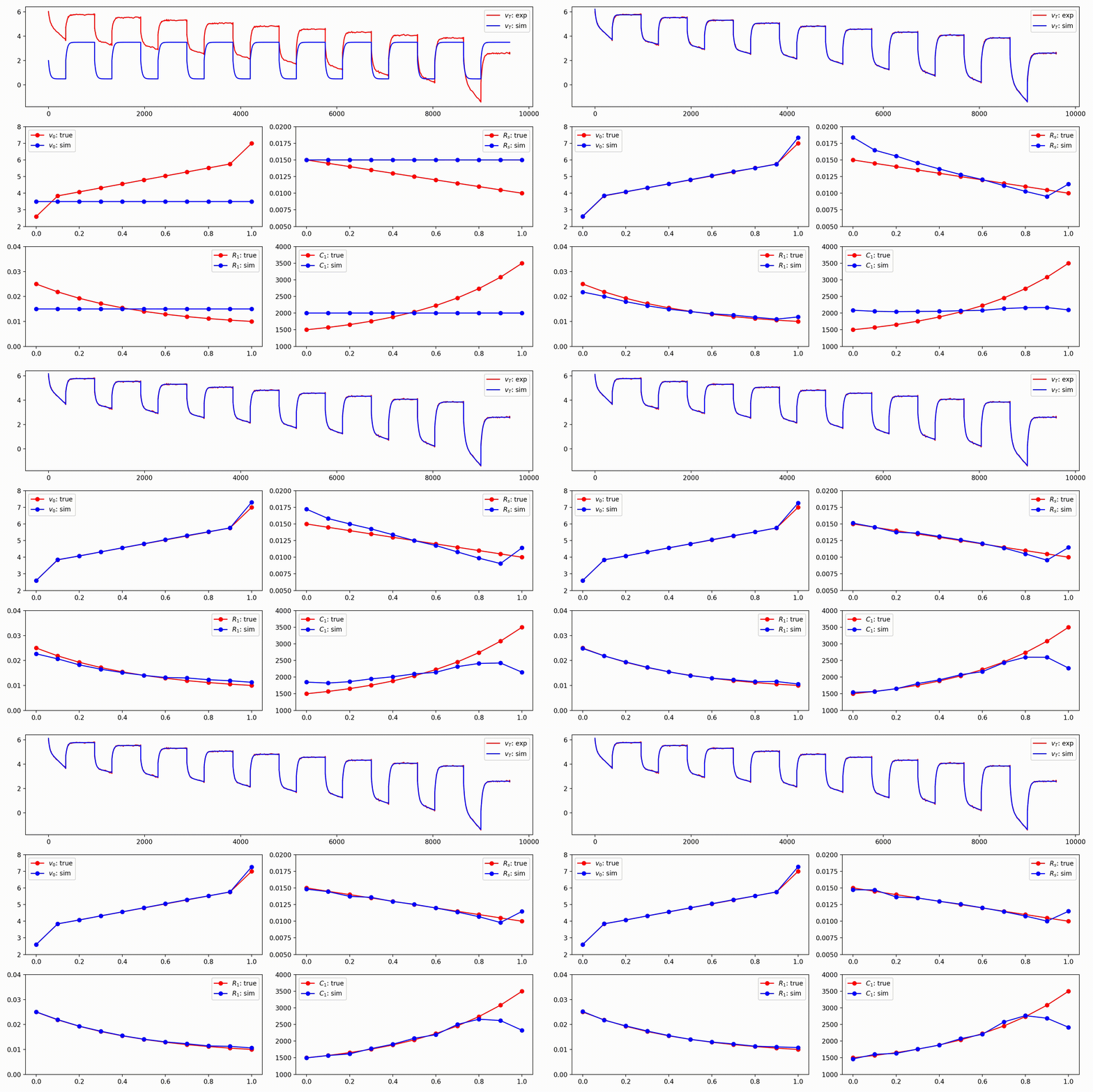

</div>

Jaxonomy can differentiate through complete simulations to fit model parameters to data — no finite-difference approximations, no hand-written adjoint code. Here we recover a spring–damper's stiffness and damping by differentiating the whole rollout and descending with Optax:

import jax
import jax.numpy as jnp
import optax
import jaxonomy as jx

class SpringDamper(jx.LeafSystem):
    def __init__(self, k=1.0, c=0.3, **kwargs):
        super().__init__(**kwargs)
        self.declare_dynamic_parameter("k", k)
        self.declare_dynamic_parameter("c", c)
        self.declare_continuous_state(
            default_value=jnp.array([1.0, 0.0]), ode=self._ode
        )

    def _ode(self, time, state, *inputs, **params):
        x, v = state.continuous_state
        return jnp.array([v, -params["k"] * x - params["c"] * v])

sd   = SpringDamper(name="sd")
opts = jx.SimulatorOptions(enable_autodiff=True, max_major_steps=200)

def final_state(theta):                       # theta = {"k": ..., "c": ...}
    ctx = sd.create_context()
    ctx.parameters["k"], ctx.parameters["c"] = theta["k"], theta["c"]
    res = jx.simulate(sd, ctx, (0.0, 1.5), options=opts)
    return res.context.continuous_state       # differentiable final [x, v]

target = jax.lax.stop_gradient(final_state({"k": 4.0, "c": 0.5}))  # "measured"
loss   = lambda theta: jnp.sum((final_state(theta) - target) ** 2)

theta   = {"k": 1.0, "c": 0.1}
opt     = optax.adam(2e-1)
state   = opt.init(theta)
grad_fn = jax.jit(jax.grad(loss))             # gradient through the ODE solver
for _ in range(300):
    updates, state = opt.update(grad_fn(theta), state)
    theta = optax.apply_updates(theta, updates)
# theta → {"k": 4.00, "c": 0.50}

jax.grad(loss) flows back through every ODE step automatically, so the same recipe scales to battery ECMs (above), powertrains, or any parametric model — and jaxonomy.optimization wraps it in a higher-level Optimizable API when you want bounds, transforms, and constraints.

---

4 · Acausal Physical Modeling

<div align="center">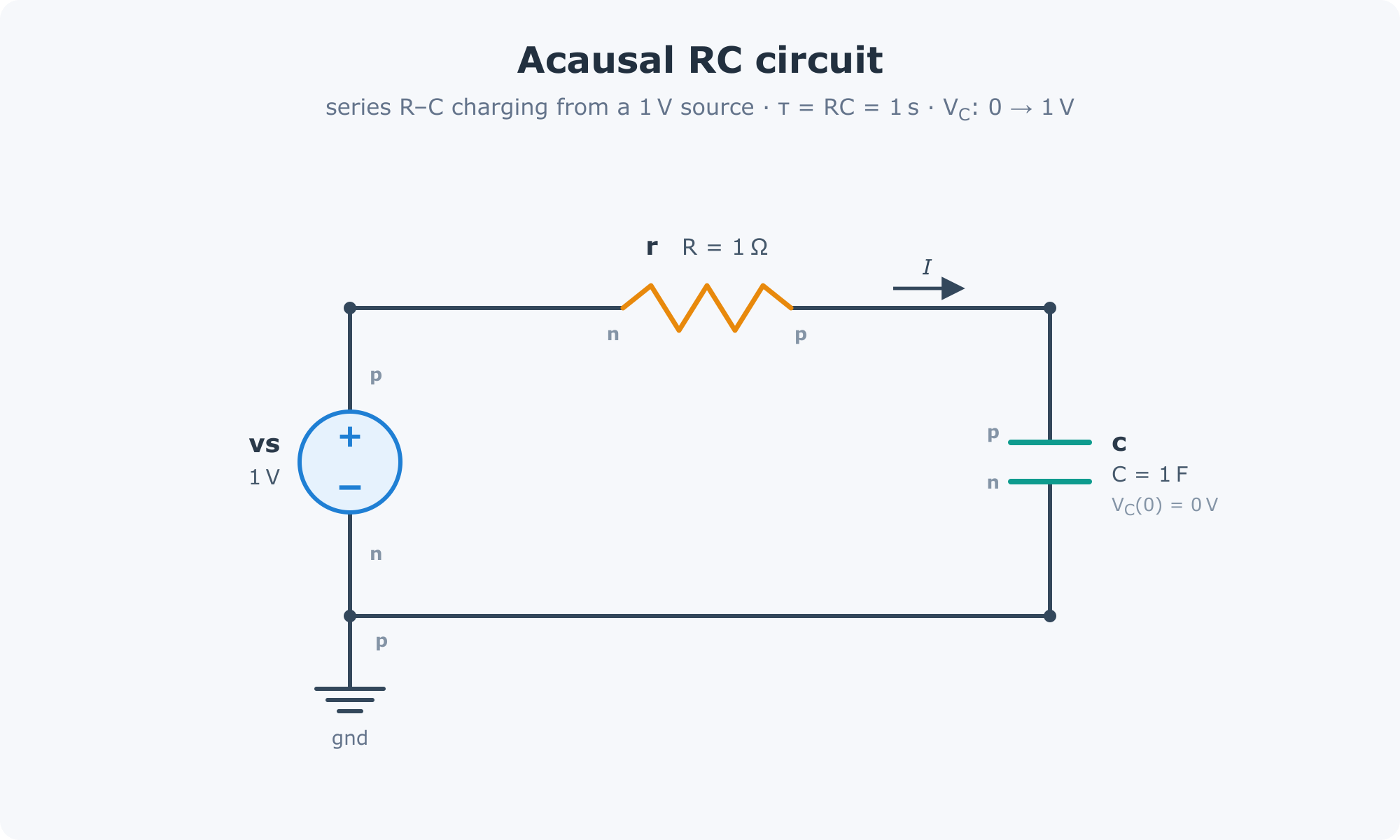

</div>

Jaxonomy includes a Modelica-inspired acausal modeling layer for multi-domain physical systems. You describe component connections symbolically; the compiler automatically derives the governing DAE, reduces its index, and emits a LeafSystem ready to drop into any diagram.

RC circuit with initial conditions:

$$ C,\dot{V}C = I, \qquad V_C(0) = 0,\text{V}, \qquad V{\text{src}} = 1,\text{V} $$

import jaxonomy as jx
from jaxonomy.acausal import AcausalCompiler, AcausalDiagram, EqnEnv
from jaxonomy.acausal import electrical as elec

ev = EqnEnv()
ad = AcausalDiagram()

vs  = elec.VoltageSource(ev, name="vs", v=1.0)
r   = elec.Resistor(ev,      name="r",  R=1.0)
c   = elec.Capacitor(ev,     name="c",  C=1.0,
                              initial_voltage=0.0, initial_voltage_fixed=True)
gnd = elec.Ground(ev,        name="gnd")

ad.connect(vs, "p", r,  "n")
ad.connect(r,  "p", c,  "p")
ad.connect(c,  "n", vs, "n")
ad.connect(vs, "n", gnd, "p")

compiler = AcausalCompiler(ev, ad)
rc_block = compiler()         # → LeafSystem, JIT-compiled ODE

builder = jx.DiagramBuilder()
rc = builder.add(rc_block)
diagram = builder.build()
results = jx.simulate(
    diagram,
    diagram.create_context(),
    (0.0, 5.0),
    recorded_signals={"rc": rc.output_ports[0]},
)

results.outputs["rc"]   # capacitor charges 0 → 0.993 V over 5 τ (R = C = 1)

The same pipeline handles multi-domain systems — an electro-mechanical actuator connecting electrical, rotational, and translational domains compiles to a single optimized system.

Available acausal domains: electrical · rotational · translational · thermal · fluid

---

5 · Differentiable Sensitivity & Batch Simulation

<div align="center">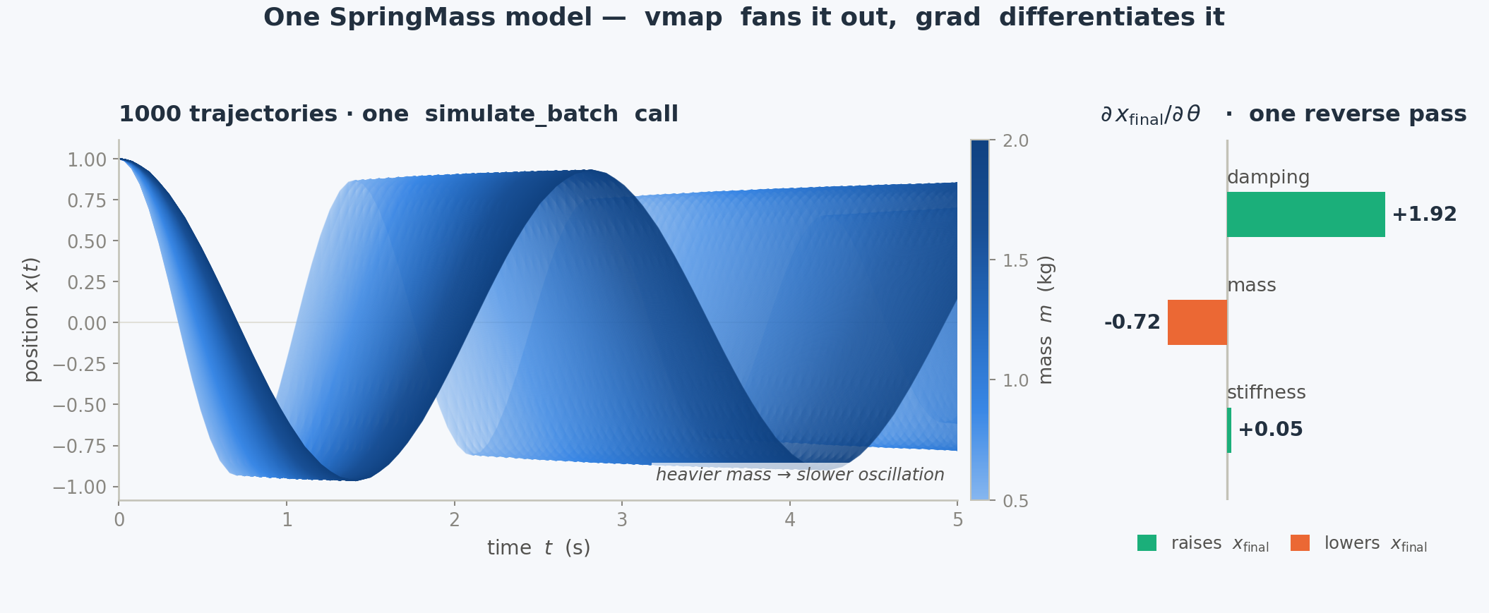

</div>

Because jax.grad, jax.jit, and jax.vmap all compose with simulate, you get powerful workflows with minimal boilerplate:

import jax
import jax.numpy as jnp
import jaxonomy as jx

class SpringMass(jx.LeafSystem):
    def __init__(self, mass=1.0, damping=0.1, stiffness=10.0, **kwargs):
        super().__init__(**kwargs)
        self.declare_dynamic_parameter("mass", mass)
        self.declare_dynamic_parameter("damping", damping)
        self.declare_dynamic_parameter("stiffness", stiffness)
        self.declare_continuous_state(
            default_value=jnp.array([1.0, 0.0]), ode=self._ode
        )
        self.declare_continuous_state_output(name="x")

    def _ode(self, time, state, *inputs, **params):
        x, v = state.continuous_state
        a = -(params["stiffness"] * x + params["damping"] * v) / params["mass"]
        return jnp.array([v, a])

# ── Sensitivity: ∂(final position)/∂(all parameters) in one reverse pass ─────
plant = SpringMass(name="plant")
grad_opts = jx.SimulatorOptions(enable_autodiff=True, max_major_steps=200)

def final_position(theta):
    ctx = plant.create_context()
    for name, value in theta.items():
        ctx.parameters[name] = value
    res = jx.simulate(plant, ctx, (0.0, 5.0), options=grad_opts)
    return res.context.continuous_state[0]

grads = jax.grad(final_position)({"mass": 1.0, "damping": 0.1, "stiffness": 10.0})

# ── Monte Carlo ensemble: 1000 trajectories over a mass sweep (vmap) ─────────
builder = jx.DiagramBuilder()
plant_b = builder.add(SpringMass(name="plant"))
diagram = builder.build()

results = jx.simulate_batch(
    diagram, t_span=(0.0, 5.0),
    param_batches={"plant.mass": jnp.linspace(0.5, 2.0, 1000)},
    options=jx.SimulatorOptions(math_backend="jax", max_major_steps=200),
    recorded_signals={"x": plant_b.output_ports[0]},
)
# results.outputs["x"] shape: (1000, T, 2)

---

🧩 Library Overview

Over 150 built-in blocks covering the full signal-processing and control toolkit. A representative slice — not exhaustive:

Category	Blocks
Sources	Constant, Step, Ramp, Chirp, Pulse, Sawtooth, Clock, DataSource
Stochastic	RandomNumber, UniformRandomNumber, WhiteNoise, BandLimitedNoise, PRBS, RandomSource — all support with_key for independent noise streams under vmap
Arithmetic & nonlinearities	Adder, Gain, Product, Abs, Power, Trigonometric, Saturate / SoftSaturate, DeadZone, RateLimiter / SoftRateLimiter, Quantizer, Backlash
Continuous dynamics	Integrator, Derivative, TransferFunction, LTISystem, PID / PIDContinuous
Discrete dynamics	IntegratorDiscrete, UnitDelay, FilterDiscrete, LowPassDiscrete, LeadLag, Notch, PIDDiscrete, PIDController2DOF, Decimator, RateTransition
Routing, buses, matrix	Mux / Demux, BusCreator / BusSelector / BusUpdate (with BusUnit annotations), Slice, Stack, Switch / MultiPortSwitch, IfThenElse, MatrixMultiplication, MatrixInversion, DotProduct, CrossProduct
Logic & state machines	TruthTable, LogicalOperator, Comparator, Relay, EdgeDetection, StateMachine (authored via StateMachineBuilder DSL)
Lookup tables	LookupTable1d / LookupTable2d / LookupTableND, Prelookup / InterpolationUsingPrelookup, TableSearch — all differentiable and fittable from data via fit_lookup_table_*
Delays & containers	TransportDelay, VariableTransportDelay, EnabledSubsystem, TriggeredSubsystem, ForEach, Conditional
Control	LinearQuadraticRegulator / DiscreteTimeLinearQuadraticRegulator / FiniteHorizonLinearQuadraticRegulator / LinearQuadraticGaussian, LinearDiscreteTimeMPC (native + LinearDiscreteTimeMPC_OSQP), DirectShootingNMPC / DirectTranscriptionNMPC / HermiteSimpsonNMPC
Estimation	KalmanFilter, ExtendedKalmanFilter, UnscentedKalmanFilter, InfiniteHorizonKalmanFilter, RecursiveLeastSquares, AugmentedStateEKF, Luenberger
Physics & coordinates	CoordinateRotation, RigidBody, BatteryCell
ML / Data	MLP (Equinox), Sindy, PyTorch, TensorFlow, ONNX / ONNXJax
ROM & surrogates	reduce(...) → ReducedOrderModel; linear MOR (balred / minreal / modal_truncation / residualize), galerkin_reduce + deim (POD–DEIM), dmd / dmdc / era, DMDForecaster / KoopmanPredictor, and surrogate blocks GaussianProcess / PolynomialChaos / RadialBasisSurrogate
Interop	ModelicaFMU / ModelicaFMUME (FMI 2.0 / 3.0 co-simulation and model-exchange import) + FMU export via build_fmu; MuJoCo / MJX; Ros2Publisher / Ros2Subscriber; QuanserHAL; PyTwin
Custom	CustomPythonBlock, CustomJaxBlock for user-authored algorithms with persistent per-instance state

Custom blocks are first-class beyond the wrappers above: subclass LeafSystem, declare ports and states, and your block integrates with the full framework including JIT, autodiff, and event detection.

---

🏗️ System Architecture

A Jaxonomy model is a Diagram — a directed graph of interconnected blocks. Blocks (LeafSystem) declare ports, continuous/discrete states, and event guards. The simulator orchestrates ODE integration, discrete updates, and event detection automatically.

graph LR
    subgraph Diagram["DiagramBuilder.build()"]
        direction LR
        r[/"r(t)\nReference"/] --> sum(("Σ"))
        sum -->|"e(t)"| ctrl["Controller\nLQR · MPC · PID"]
        ctrl -->|"u(t)"| plant["Plant\nLTI · Nonlinear · Acausal"]
        plant -->|"x(t)"| obs["State Estimator\nKalman · EKF · UKF"]
        obs --> sum
        plant -->|"y(t)"| out[/"y(t)\nOutput"/]
    end

    style Diagram fill:#f5f8ff,stroke:#4a6fa5,stroke-width:2px
    style ctrl fill:#dbeafe,stroke:#2563eb
    style plant fill:#dcfce7,stroke:#16a34a
    style obs fill:#fef9c3,stroke:#ca8a04

The JAX backend sits underneath every simulation, giving you a clean Python API backed by XLA compilation:

graph TD
    A["Python API\nDiagram · LeafSystem · simulate()"] --> B["JAX Backend\nJIT · vmap · grad"]
    B --> C1["Dopri5\nAdaptive RK45\nnon-stiff ODEs"]
    B --> C2["BDF\nImplicit solver\nstiff systems"]
    B --> C3["Event Handler\nZero-crossing\nbisection"]

    style A fill:#e0f2fe,stroke:#0284c7
    style B fill:#fdf4ff,stroke:#9333ea
    style C1 fill:#f0fdf4,stroke:#16a34a
    style C2 fill:#f0fdf4,stroke:#16a34a
    style C3 fill:#f0fdf4,stroke:#16a34a

---

The Jaxonomy stack

Jaxonomy is the engine at the base of a three-package stack. Each package is its own repository, MIT-licensed, and depends only on the package(s) above it:

• Jaxonomy — this package. The general-purpose, JAX-native simulation engine for hybrid dynamical systems. Not robotics-specific; depends on nothing else in the stack.
• Jaxterity — the robotics layer built on top of Jaxonomy: URDF/MJCF import, MJX-backed articulated dynamics, calibrated actuators/sensors, system identification, and whole-body control. Imports Jaxonomy; never re-implements its primitives.
• Jaxility — the deployment artifact factory: compiles a calibrated robot to embedded C for Arm SoCs (Cortex-A / Cortex-M) with a signed attestation manifest. Consumes Jaxterity.

The boundary rule: anything useful to controls engineers outside robotics (HVAC, battery, aerospace, energy) belongs in Jaxonomy; anything specific to joints, actuators, contacts, and kinematic chains belongs in Jaxterity; embedded codegen, targets, and attestation belong in Jaxility.

What Jaxonomy does not yet do (or does only partially) is tracked in KNOWN_GAPS.md — the public inverse of the internal evidence ledger in CLAIMS.md.

License

Released under the MIT License from version 2.2.0 onward.

Derived from the MIT-licensed open-source package pycollimator by Collimator, Inc. </content> </invoke>